______________________________________________________________________________________________________________________________________

Introduction

Online Social Networks are becoming increasingly popular as a tool for collaboration and communication as it provides a common platform to connect millions of Internet users. However, several studies show that these networks provide an effective mechanism for spreading phishing attacks, spam campaigns and even fake news. Spammers all around the globe are progressively relying on such networks for propagating spam among the members of this virtual community. The social networks provides liberty to the users to contribute any amount of content freely. Since, millions of users at connected with each others, the rate of propagation of information is much higher as compared to traditional forms of communication like email, SMS, etc. This encourages the spammers to exploit these networks for their benefits. The extensive rise of social media and increase in global connections further elevate the extent of spread. So, a framework is required which distinguishes spam messages from the legitimate ones (ham messages).

Spam: An unwanted, junk, unsolicited message used for spreading misinformation, malicious content, advertisements, etc in order to gain profit at a negligible cost.

Ham: A legitimate, wanted or solicited message. It is a message that is generally desired and isn’t considered as spam.

In this project, a basic framework is developed for classification of messages into HAM or SPAM. This is done by training a model using freely available datasets for academic and research purposes. R has been used as the statistical computing environment to carry out the necessary analysis. A detailed stepwise approach has been illustrated to process the dataset and build the classification model. Further, the performance of the model is also evaluated by testing it on a set on unseen messages and comparing the predicted results with the true labels.

Introduction to Classification

Classification is a type of predictive modelling. It comprises of assigning a class label to a set of unclassified instances. It involves building of a model which has the ability to predict the category which the given given data belongs to.

In context of this project, two major steps are involved in classification:

1. Setting up the model

• Every data sample is assumed to belong to a predefined class, as determined by its respective label.
• A set of pre-classified instances is used as a training set to build the classification model.
• There are several ways to represent this model, i.e., classification rules, decision trees, or mathematical formulae.

2. Testing and usage of the model

• The accuracy of the model is evaluated by testing it on a set of unseen data points and comparing the results with the true labels.
• If the model exhibits acceptable accuracy, it can be then used to classify new set of data points.

Description of the dataset

The dataset is a data frame structure containing 5559 observations (number of messages) each with two columns, the “type” column that indicates whether the message is a SPAM (trashed) message or a HAM (legitimate) message, and the “text” column that contains the actual message content. This is an open dataset and can be downloaded from the link: https://www.kaggle.com/vivekchutke/spam-ham-sms-dataset

Step-wise approach for building and testing the classification model

The first step is to load the dataset into the environment.

Step 1: Reading the dataset into the environment for analysis.

Step 2: Examining the structure of the dataset to identify the variables and their types.

It can be clearly seen that the given dataset contains two columns which are both character data. For the “type” attribute to be used as a classifier label for classifying the messages as HAM or SPAM, it has to be converted into a factor vector.

Step 3: Converting ham/spam into factors and re-examining the structure.

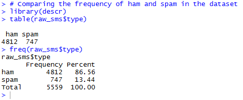
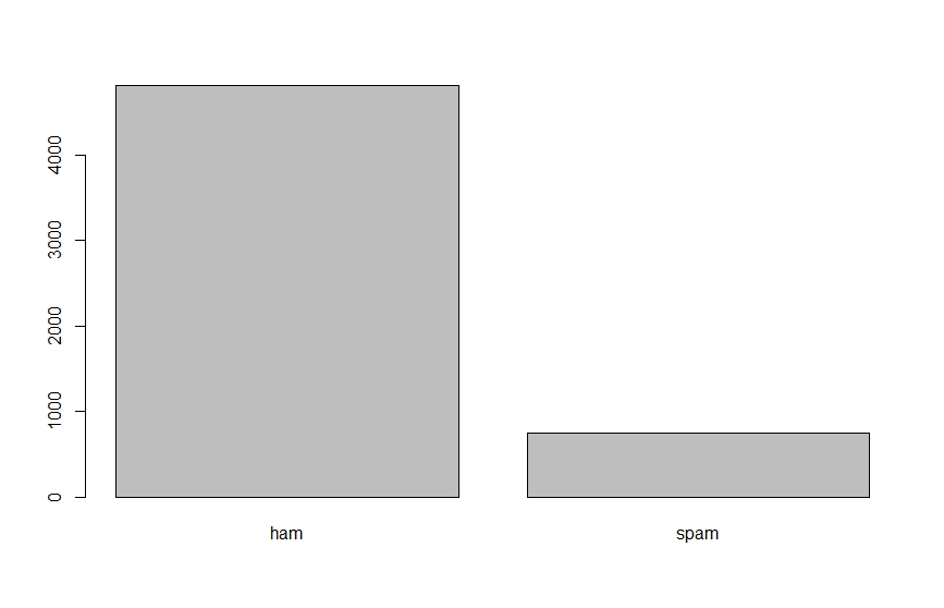
Step 4: Comparing frequency of ham and spam in the dataset.

Now, the text data cannot be dealt with directly in a data frame structure, it needs to be converted into a volatile corpus. It is basically a text document with information of all the messages in the dataset in a short term memory.

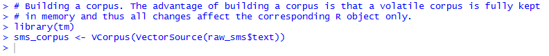
Step 5: Building a corpus. The advantage of building a corpus is that a volatile corpus is fully kept in memory and thus all changes affect the corresponding R object only.

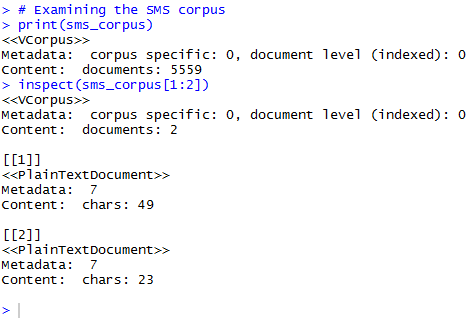
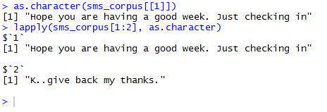
A quick glance at the VCorpus information can be obtained in terms of number of documents (similar to number of messages) in a metadata through the use of inspect() command. The actual content can also be accessed through the use of as.character().

Step 6: Examining the SMS corpus.

Currently, the data in the corpus is in a raw format. Before analysing the data, some pre-processing tasks have to be performed. These include changing all possible capital letters in lower cases, removal of numerical value that neither indicate spam nor ham; removal of a list of stop words such as “a”, “an”, “the”, “for”, “is”, etc. which neither indicate spam nor ham, removal of any punctuation, performing word stemming, stripping away the unnecessary white spaces and so on. The tm_map() function provides a method to apply the aforementioned transformations (also known as mappings) to a volatile corpus.

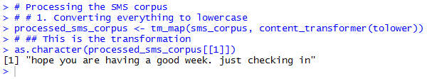
Step 7: Processing the SMS Corpus.

7.1 Converting everything to lowercase.

7.2 Removing numbers.

7.3 Removing stopwords.

7.4 Removing punctuation.

7.5 A custom function can also be made to replace punctuation rather than removing it.

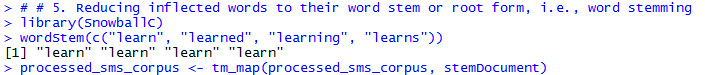
7.6 Reducing inflected words to their word stem or root form, i.e., word stemming. The tm package provides stemming functionality via integration with the SnowballC package.

7.7 Removing unnecessary white spaces.

Now, the next step is to split each of the messages in the dataset into individual components. This process is called tokenization. A token is a single element of a text string. In this case, a token represents a word in a message.

The DocumentTermMatrix() function accepts a corpus as input and creates a data structure called a Document Term Matrix (DTM) in which rows indicate documents (i.e., messages) and columns indicate terms (i.e., words).

Applying the function on the processed corpus will lead to creation of a sms_dtm_sprs object which contains the tokenized corpus using the default settings, applying minimal processing. The default settings are appropriate because the corpus has already been prepared manually.

However, if pre-processing wouldn’t have been performed manually earlier as shown in the above steps, it could also be done here by providing a list of control parameters options so as to override the defaults.

Step 8: Creating a document-term sparse matrix directly from the SMS corpus.

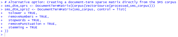
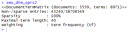
Note: The DocumentTermMatrix() function applies its cleanup functions to the text strings only after the individual messages have been split apart into words. Thus, it uses a slightly different stop words removal function.

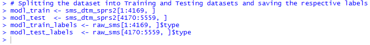
The dataset is now ready for analysis after completion of all the pre-processing tasks. The next step is to split the processed dataset into two parts, one for training and the other for testing. This is done so that once the message classifier is built, its performance can be evaluated on data that has not been encountered previously. It is to be noted here that the split is occuring after the entire data have been cleaned and processed. The same preparation steps are required to take place on both the training and test datasets. Here, 75% of the data has been used for training and 25% for testing. Since the messages are sorted in a random order, the first 4,169 rows have been considered for training and the remaining 1,390 for testing.

Step 9: Splitting the dataset into Training and Testing datasets and saving the respective labels.

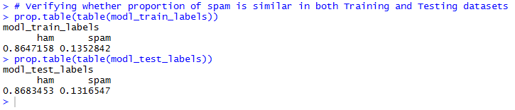
Step 10: Verifying whether proportion of spam is similar in both Training and Testing datasets.

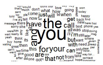
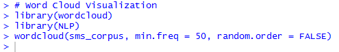
A word cloud is a way to visually depict the frequency at which words appear in a given text data. The cloud is composed of several words scattered randomly over the entire figure. Words appearing more often in the text are depicted in a larger font, while less common words are depicted in smaller fonts.

Step 11: Word Cloud Visualisation for the entire corpus.

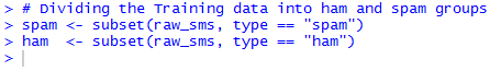
A more interesting visualisation involves comparing the word clouds of HAM and SPAM groups.

Step 12: Dividing the Training data into ham and spam groups.

Step 13: Word Cloud Visualisation for spam and ham groups separately.

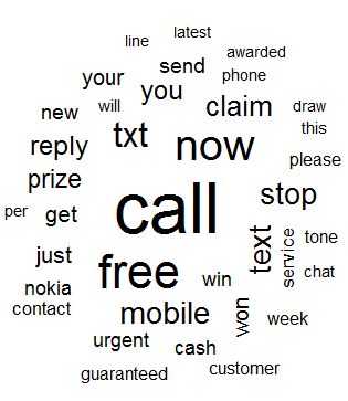
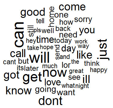
Spam messages include words such as urgent, free, mobile, claim, guaranteed and stop. On the contrary, these terms do not appear in the ham cloud at all. Instead, ham messages comprise of words such as can, sorry, need, home and time. These stark differences suggest that the model to be developed will have some strong key words to differentiate between the two message classes.

The next step in the data preparation process in to transform the sparse document term matrix into a data structure that can be used to train the message classifier. Presently, the sparse matrix might incorporate a very large number of features, may be a feature for every word that appears in at least one message in the entire dataset. However, it is very unlikely that all these features would prove to be useful for classification of messages.

Step 14: Removal of sparse terms from the training dataset.

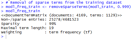
In order to reduce the number of features, any word which appears in less than five messages in the training dataset, or in less than about 0.1% of the records in the training data can be eliminated.

Step 15: Compiling frequently appearing terms in a vector.

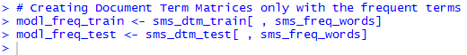
The Document Term Matrix will now be filtered to include only the frequently appearing terms, i.e., data with less number of features.

Step 16: Creating Document Term Matrices only with the frequent terms.

The Naive Bayes classifier (which would be developed for classification of messages) is typically trained on data with categorical features. This presents a problem, because the cells in the sparse matrix are numeric as it measures the number of times a word appears in the messages. So, this has to be changed into a categorical variable that simply indicates yes or no depending on whether the word appears or not. This can be done by converting the counts to factors, as shown below:

Step 17: Defining a function for converting counts to factor.

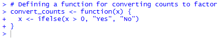
The convert_counts() function needs to be applied to each of the columns in the sparse matrix.

Step 18: Applying convert_counts() function to columns of Training and Testing data.

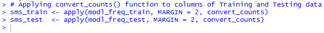
As a result of this, two character type matrices will be obtained, each with cells indicating “Yes” or “No” depending on whether the word represented by the column appears at any point in the message represented by the row in that particular matrix. At this stage, the raw messages have been converted into  a format that can be represented by a statistical model.

In this project, Naive Bayes classification algorithm is used for classification of messages into ham/spam.

The Naive Bayes classification algorithm is a probabilistic classifier based on probability models that incorporates strong independence assumptions. The crux of the classifier is based on Bayes theorem.

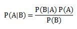
The Bayes theorem helps us to evaluate the probability of A happening, given that B has occurred. Here, B is the evidence and A is the hypothesis. The assumption made here is that the predictors/features are independent, i.e., the presence of one particular feature does not affect the others. Hence it is called “naive”.

There are two basic assumptions:

• All the predictors are independent to each other.
• All the predictors have an equal effect on the outcome.

With regards to the dataset used here, we can apply Bayes theorem in the following manner:

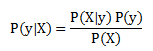
Here, y is the class variable (i.e., the message being ham or spam) and X is the dependent feature vector of size n. X = (x1, x2, x3, …, xn)

So, the above equation can be re-written as:

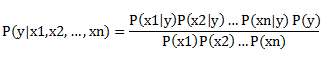
The values for each of the terms can be obtained by referring to the processed dataset, and the respective value can be substituted. For all entries in the dataset, the denominator doesn’t change, it remains constant. Hence, the denominator can be removed and proportionality can be introduced.

Now, to create a classifier model, the probability of given set of inputs for all possible values of the class variable y is found and the output with maximum probability has to be selected. In case of the dataset considered here, the class variable has only two possible outcomes: HAM or SPAM. This can be expressed mathematically as:

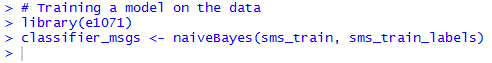
Given the predictors, the class of messages can be computed using the above function. Now, a model will be trained using Naive Bayes classification algorithm.

Step 19: Training a model on the data.

To evaluate the performance of the model, its predictions need to be tested on unseen messages in the Testing dataset. The classifier would be used to generate predictions and then, the predicted values will be compared against the true values.

Step 20: Testing the performance of the model.

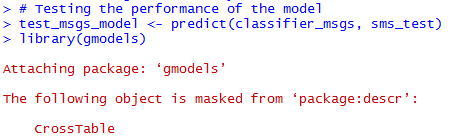
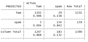
Step 21: The results are compiled in the form of a confusion matrix.

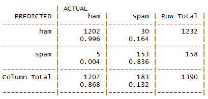
By referring to the above table, we can easily make out that only 35 messages out of a total of 1390 messages are misclassified. In the set of errors, there are 5 out of 1207 HAMs, which are misclassified as SPAMs, and 30 out of 183 SPAMs are misclassified as HAMs. The accuracy for each of the cases is also highlighted in the confusion matrix.  The overall accuracy of the model is about 97.48%, which is quite impressive.

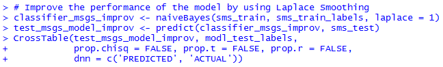
The performance of the algorithm can be improved by implementing Laplace Smoothing in Naive Bayes classifier. This can be done by setting a true value for the Laplace estimator while training the model. This basically allows for the words that didn’t appear in any of the HAM or SPAM messages to have an indisputable say in the classification process.

Step 22: Attempting to improve the performance of the model by using Laplace Smoothing.

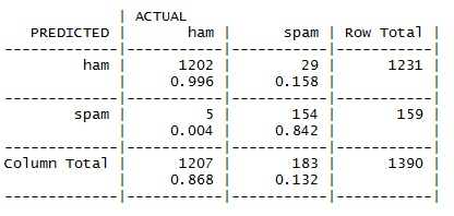
By referring to the above table, we can easily make out that only 34 messages out of a total of 1390 messages are misclassified. The number of misclassified HAMs is same as that in the previous case. However, the number of misclassified SPAMs is reduced by 1. The overall accuracy of the model is about 97.55%, which is a bit higher as compared to the previous case.

Extensions of the work

Categorisation of spam messages

There are several categories of SPAMs which are encountered in everyday lives, like health spams, finance-based spams, education spams (predatory journals and illegitimate publishers), advertisements, and so on. An extensive dataset can be created containing sufficient numbers of each of the spam categories collected from several inboxes. A model can then be trained to categorise the spam messages into various categories, as elucidated earlier. Such a model would be of great interest to social scientists and data analysts, as it would not only tell whether a message is spam or not, but it will also reflect upon the category of spam which it belongs to.

Fake News

Fake news is often referred to as a type of ‘yellow journalism’ or ‘propaganda deliberate misinformation’ or ‘hoaxes’ spread using multimedia. Some of the primary motives include increasing readership, online sharing and internet click revenue. The extensive rise of social media and increase in global connections further elevate the extent spread. The main intent of broadcasting fake news is to mislead the masses. This promptly helps several individuals and organisations gain financially or politically, due to exaggerated or patently false headlines that grab attention. One of the major drawbacks of unnecessary fake news is that it undermines serious media coverage and makes it more difficult for the media professionals to cover authentic and significant news stories.

A significant portion of the population today, especially the youngsters get their news from social media, which turns out to be the most prominent place for fake news to spread easily. The giant like Facebook, Twitter, WhatsApp and other social media platforms are built to easily share information with the connections. The content being shared through these platforms is not censored or verified to ensure its truthfulness. This virtually signifies that almost any content, regardless of any specific parameter, can be shared very easily and can quickly go viral, though it is fake.

In all the social media platforms, several machine learning algorithms are implemented, due to which users are shown content based on their likes and preferences. Although this content curation shows us things that we like to see, it greatly limits the diversity of our news sources and even distorts our perception of differentiating between the true and fake content. This often aids in reinforcing our existing beliefs and doesn’t allow the individuals to dig deeper and ponder over the content we are reading and to see both pros and cons of an issue.

It is quite difficult to spot a content or link containing fake news. Several of the fake articles are published by look-alike websites specifically designed to make the user believe firmly that he/she is reading the said content from a trustworthy source. A lot of online falsehoods are being made to look legitimate through sophisticated machinery, with bots and fake accounts that like, retweet and comment on fake news. Social media makes the problem worse because of its social factor, whereby being the first to share breaking news thought to be of interest to one’s friends may be seen as something welcomed.

The basic classification framework can be extended with much more capabilities for online classification of a news piece. If a particular news article is detected to be fake, its spread can be eliminated in the entire network and masses won’t get exposed to misinformation generated from the fraudulent sources.

References

1. Gao, H., Chen, Y., Lee, K., Palsetia, D., & Choudhary, A. N. (2012, February). Towards Online Spam Filtering in Social Networks. In NDSS (Vol. 12, No. 2012, pp. 1-16).

2. Wang, D., Irani, D., & Pu, C. (2011, September). A social-spam detection framework. In Proceedings of the 8th Annual Collaboration, Electronic messaging, Anti-Abuse and Spam Conference (pp. 46-54). ACM.

3. Zhang, X., Zhu, S., & Liang, W. (2012, December). Detecting spam and promoting campaigns in the twitter social network. In 2012 IEEE 12th international conference on data mining (pp. 1194-1199). IEEE.

4. Chakraborty, M., Pal, S., Pramanik, R., & Chowdary, C. R. (2016). Recent developments in social spam detection and combating techniques: A survey. Information Processing & Management, 52(6), 1053-1073.

5. Jeong, S., Noh, G., Oh, H., & Kim, C. K. (2016). Follow spam detection based on cascaded social information. Information Sciences, 369, 481-499.

6. YouTube video on Email Spam Detection. Link: https://www.youtube.com/watch?v=sQfct3xuQIE&t=61s

______________________________________________________________________________________________________________________________________

Appendix

Complete code implemented in R

# Deepesh Agarwal (18250010)

# Digital Cultures and New Media - Project

# Reading the dataset
raw_sms <- read.csv("E:/dcnm_project/sms_spam.csv", stringsAsFactors = FALSE)

# Examining the structure of the dataset
str(raw_sms)

# Converting ham/spam into factors and re-examining the structure
raw_sms$type <- factor(raw_sms$type)
str(raw_sms)

# Comparing the frequency of ham and spam in the dataset
library(descr)
table(raw_sms$type)
freq(raw_sms$type)

# Building a corpus. The advantage of building a corpus is that a volatile corpus is fully kept
# in memory and thus all changes affect the corresponding R object only.
library(tm)
sms_corpus <- VCorpus(VectorSource(raw_sms$text))

# Examining the SMS corpus
print(sms_corpus)
inspect(sms_corpus[1:2])

as.character(sms_corpus[[1]])
lapply(sms_corpus[1:2], as.character)

# Processing the SMS corpus
# # 1. Converting everything to lowercase
processed_sms_corpus <- tm_map(sms_corpus, content_transformer(tolower))
# ## This is the transformation
as.character(processed_sms_corpus[[1]])
# # 2. Removing numbers
processed_sms_corpus <- tm_map(processed_sms_corpus, removeNumbers)
# # 3. Removing stop words
processed_sms_corpus <- tm_map(processed_sms_corpus, removeWords, stopwords())
# # 4. Removing punctuation
processed_sms_corpus <- tm_map(processed_sms_corpus, removePunctuation)
# ## A custom function can also be made to replace punctuation rather than removing it
replacePunctuation <- function(x) { gsub("[[:punct:]]+", " ", x) }
processed_sms_corpus <- replacePunctuation(processed_sms_corpus)
# # 5. Reducing inflected words to their word stem or root form, i.e., word stemming
library(SnowballC)
wordStem(c("learn", "learned", "learning", "learns"))
processed_sms_corpus <- tm_map(processed_sms_corpus, stemDocument)
# # 6. Removing unnecessary white spaces
processed_sms_corpus <- tm_map(processed_sms_corpus, stripWhitespace)
# Alternative option: Creating a document-term sparse matrix directly from the SMS corpus
sms_dtm_sprs <- DocumentTermMatrix(Corpus(VectorSource(processed_sms_corpus)))
sms_dtm_sprs2 <- DocumentTermMatrix(sms_corpus, control = list(
tolower = TRUE,
removeNumbers = TRUE,
stopwords = TRUE,
removePunctuation = TRUE,
stemming = TRUE
))
sms_dtm_sprs
sms_dtm_sprs2
class(sms_dtm_sprs2)
as.character(sms_dtm_sprs[[1]])

# Splitting the dataset into Training and Testing datasets and saving the respective labels
modl_train <- sms_dtm_sprs2[1:4169, ]
modl_test <- sms_dtm_sprs2[4170:5559, ]
modl_train_labels <- raw_sms[1:4169, ]$type
modl_test_labels <- raw_sms[4170:5559, ]$type

# Verifying whether proportion of spam is similar in both Training and Testing datasets
prop.table(table(modl_train_labels))
prop.table(table(modl_test_labels))

# Word Cloud Visualization for the entire corpus
library(wordcloud)
library(NLP)
wordcloud(sms_corpus, min.freq = 50, random.order = FALSE)

# Dividing the Training data into ham and spam groups
spam <- subset(raw_sms, type == "spam")
ham <- subset(raw_sms, type == "ham")

# Word Cloud Visualization for spam and ham groups separately
wordcloud(spam$text, min.freq = 20, random.order = FALSE)
wordcloud(ham$text, min.freq = 20, random.order = FALSE)

# Removal of sparse terms from the training dataset
modl_freq_train <- removeSparseTerms(modl_train, 0.999)
modl_freq_train

# Frequent terms
findFreqTerms(modl_train, 5)

# Compiling frequently appearing terms in a vector
sms_freq_words <- findFreqTerms(modl_train, 5)
str(sms_freq_words)

# Creating Document Term Matrices only with the frequent terms
modl_freq_train <- sms_dtm_train[ , sms_freq_words]
modl_freq_test <- sms_dtm_test[ , sms_freq_words]

# Defining a function for converting counts to factor
convert_counts <- function(x) {
x <- ifelse(x > 0, "Yes", "No")
}

# Applying convert_counts() function to columns of Training and Testing data
sms_train <- apply(modl_freq_train, MARGIN = 2, convert_counts)
sms_test <- apply(modl_freq_test, MARGIN = 2, convert_counts)

# Training a model on the data
library(e1071)
classifier_msgs <- naiveBayes(sms_train, sms_train_labels)

# Testing the performance of the model
test_msgs_model <- predict(classifier_msgs, sms_test)
library(gmodels)
CrossTable(test_msgs_model, modl_test_labels,
prop.chisq = FALSE, prop.t = FALSE, prop.r = FALSE,
dnn = c('PREDICTED', 'ACTUAL'))

# Improve the performance of the model by using Laplace Smoothing
classifier_msgs_improv <- naiveBayes(sms_train, sms_train_labels, laplace = 1)
test_msgs_model_improv <- predict(classifier_msgs_improv, sms_test)
CrossTable(test_msgs_model_improv, modl_test_labels,
prop.chisq = FALSE, prop.t = FALSE, prop.r = FALSE,
dnn = c('PREDICTED', 'ACTUAL'))

______________________________________________________________________________________________________________________________________